Introducing Shiny
Shiny is a new package from RStudio that makes it incredibly easy to build interactive web applications with R.
For an introduction and live examples, visit the Shiny homepage.
Features
- Build useful web applications with only a few lines of code—no JavaScript required.
- Shiny applications are automatically “live” in the same way that spreadsheets are live. Outputs change instantly as users modify inputs, without requiring a reload of the browser.
- Shiny user interfaces can be built entirely using R, or can be written directly in HTML, CSS, and JavaScript for more flexibility.
- Works in any R environment (Console R, Rgui for Windows or Mac, ESS, StatET, RStudio, etc.)
- Attractive default UI theme based on Twitter Bootstrap.
- A highly customizable slider widget with built-in support for animation.
- Pre-built output widgets for displaying plots, tables, and printed output of R objects.
- Fast bidirectional communication between the web browser and R using the websockets package.
- Uses a reactive programming model that eliminates messy event handling code, so you can focus on the code that really matters.
- Develop and redistribute your own Shiny widgets that other developers can easily drop into their own applications (coming soon!).
Installation
Shiny is available on CRAN, so you can install it in the usual way from your R console:
install.packages("shiny")
Let’s Go!
This tutorial covers the basics of Shiny and provides detailed examples of using much of its capabilities. Click the Next button to get started and say hello to Shiny!
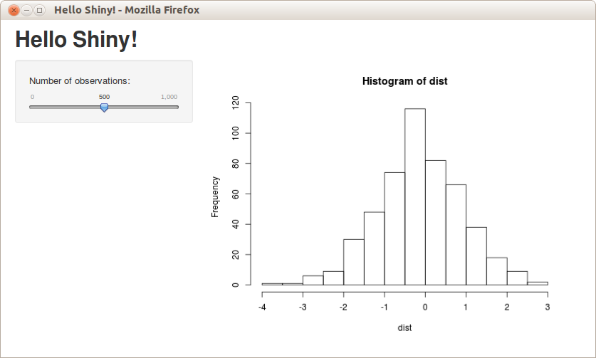
The Hello Shiny example is a simple application that generates a random distribution with a configurable number of observations and then plots it. To run the example, type:
> library(shiny)
> runExample("01_hello")
Shiny applications have two components: a user-interface definition and a server script. The source code for both of these components is listed below.
In subsequent sections of the tutorial we’ll break down all of the code in detail and explain the use of “reactive” expressions for generating output. For now, though, just try playing with the sample application and reviewing the source code to get an initial feel for things. Be sure to read the comments carefully.
The user interface is defined in a source file named ui.R:
ui.R
library(shiny)

# Define UI for application that plots random distributions
shinyUI(pageWithSidebar(

  # Application title
  headerPanel("Hello Shiny!"),

  # Sidebar with a slider input for number of observations
  sidebarPanel(
    sliderInput("obs",
                "Number of observations:",
                min = 0,
                max = 1000,
                value = 500)
  ),

  # Show a plot of the generated distribution
  mainPanel(
    plotOutput("distPlot")
  )
))
The server-side of the application is shown below. At one level, it’s very simple–a random distribution with the requested number of observations is generated, and then plotted as a histogram. However, you’ll also notice that the function which returns the plot is wrapped in a call to renderPlot. The comment above the function explains a bit about this, but if you find it confusing, don’t worry–we’ll cover this concept in much more detail soon.
server.R
library(shiny)

# Define server logic required to generate and plot a random distribution
shinyServer(function(input, output) {

  # Expression that generates a plot of the distribution. The expression
  # is wrapped in a call to renderPlot to indicate that:
  #
  #  1) It is "reactive" and therefore should be automatically
  #     re-executed when inputs change
  #  2) Its output type is a plot
  #
  output$distPlot <- renderPlot({

    # generate an rnorm distribution and plot it
    dist <- rnorm(input$obs)
    hist(dist)
  })
})
The next example will show the use of more input controls, as well as the use of reactive functions to generate textual output.
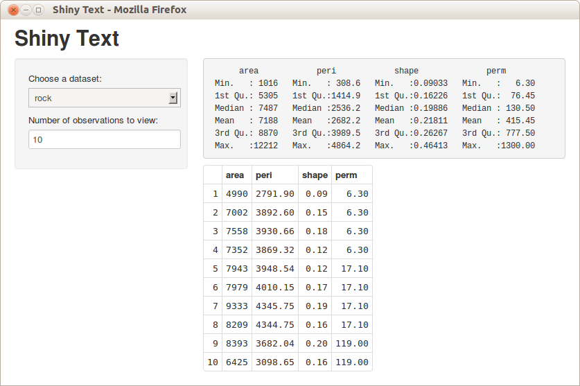
The Shiny Text application demonstrates printing R objects directly, as well as displaying data frames using HTML tables. To run the example, type:
> library(shiny)
> runExample("02_text")
The first example had a single numeric input specified using a slider and a single plot output. This example has a bit more going on: two inputs and two types of textual output.
If you try changing the number of observations to another value, you’ll see a demonstration of one of the most important attributes of Shiny applications: inputs and outputs are connected together “live” and changes are propagated immediately (like a spreadsheet). In this case, rather than the entire page being reloaded, just the table view is updated when the number of observations change.
Here is the user interface definition for the application. Notice in particular that the sidebarPanel and mainPanel functions are now called with two arguments (corresponding to the two inputs and two outputs displayed):
ui.R
library(shiny)

# Define UI for dataset viewer application
shinyUI(pageWithSidebar(

  # Application title
  headerPanel("Shiny Text"),

  # Sidebar with controls to select a dataset and specify the number
  # of observations to view
  sidebarPanel(
    selectInput("dataset", "Choose a dataset:",
                choices = c("rock", "pressure", "cars")),

    numericInput("obs", "Number of observations to view:", 10)
  ),

  # Show a summary of the dataset and an HTML table with the requested
  # number of observations
  mainPanel(
    verbatimTextOutput("summary"),

    tableOutput("view")
  )
))
The server side of the application has also gotten a bit more complicated. Now we create:
- A reactive expression to return the dataset corresponding to the user choice
- Two other rendering expressions (
renderPrintandrenderTable) that return theoutput$summaryandoutput$viewvalues
These expressions work similarly to the renderPlot expression used in the first example: by declaring a rendering expression you tell Shiny that it should only be executed when its dependencies change. In this case that’s either one of the user input values (input$dataset or input$n).
server.R
library(shiny)
library(datasets)

# Define server logic required to summarize and view the selected dataset
shinyServer(function(input, output) {

  # Return the requested dataset
  datasetInput <- reactive({
    switch(input$dataset,
           "rock" = rock,
           "pressure" = pressure,
           "cars" = cars)
  })

  # Generate a summary of the dataset
  output$summary <- renderPrint({
    dataset <- datasetInput()
    summary(dataset)
  })

  # Show the first "n" observations
  output$view <- renderTable({
    head(datasetInput(), n = input$obs)
  })
})
We’ve introduced more use of reactive expressions but haven’t really explained how they work yet. The next example will start with this one as a baseline and expand significantly on how reactive expressions work in Shiny.
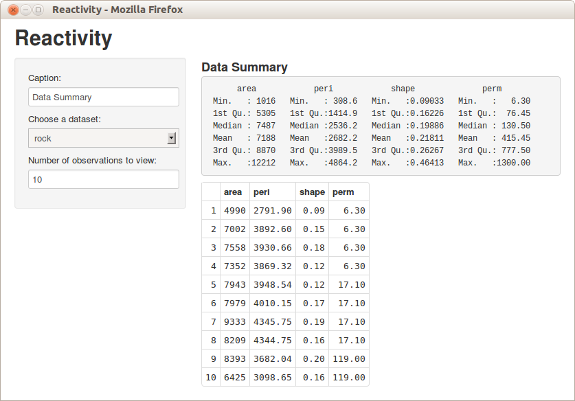
The Reactivity application is very similar to Hello Text, but goes into much more detail about reactive programming concepts. To run the example, type:
> library(shiny)
> runExample("03_reactivity")
The previous examples have given you a good idea of what the code for Shiny applications looks like. We’ve explained a bit about reactivity, but mostly glossed over the details. In this section, we’ll explore these concepts more deeply. If you want to dive in and learn about the details, see the Understanding Reactivity section, starting with Reactivity Overview.
What is Reactivity?
The Shiny web framework is fundamentally about making it easy to wire up input values from a web page, making them easily available to you in R, and have the results of your R code be written as output values back out to the web page.
input values => R code => output valuesSince Shiny web apps are interactive, the input values can change at any time, and the output values need to be updated immediately to reflect those changes.
Shiny comes with a reactive programming library that you will use to structure your application logic. By using this library, changing input values will naturally cause the right parts of your R code to be reexecuted, which will in turn cause any changed outputs to be updated.
Reactive Programming Basics
Reactive programming is a coding style that starts with reactive values–values that change over time, or in response to the user–and builds on top of them with reactive expressions–expressions that access reactive values and execute other reactive expressions.
What’s interesting about reactive expressions is that whenever they execute, they automatically keep track of what reactive values they read and what reactive expressions they invoked. If those “dependencies” become out of date, then they know that their own return value has also become out of date. Because of this dependency tracking, changing a reactive value will automatically instruct all reactive expressions that directly or indirectly depended on that value to re-execute.
The most common way you’ll encounter reactive values in Shiny is using the input object. The input object, which is passed to your shinyServer function, lets you access the web page’s user input fields using a list-like syntax. Code-wise, it looks like you’re grabbing a value from a list or data frame, but you’re actually reading a reactive value. No need to write code to monitor when inputs change–just write reactive expression that read the inputs they need, and let Shiny take care of knowing when to call them.
It’s simple to create reactive expression: just pass a normal expression into reactive. In this application, an example of that is the expression that returns an R data frame based on the selection the user made in the input form:
datasetInput <- reactive({
   switch(input$dataset,
          "rock" = rock,
          "pressure" = pressure,
          "cars" = cars)
})
To turn reactive values into outputs that can viewed on the web page, we assigned them to the output object (also passed to the shinyServer function). Here is an example of an assignment to an output that depends on both the datasetInput reactive expression we just defined, as well as input$obs:
output$view <- renderTable({
   head(datasetInput(), n = input$obs)
})
This expression will be re-executed (and its output re-rendered in the browser) whenever either the datasetInput or input$obs value changes.
Back to the Code
Now that we’ve taken a deeper loop at some of the core concepts, let’s revisit the source code and try to understand what’s going on in more depth. The user interface definition has been updated to include a text-input field that defines a caption. Other than that it’s very similar to the previous example:
ui.R
library(shiny)

# Define UI for dataset viewer application
shinyUI(pageWithSidebar(

  # Application title
  headerPanel("Reactivity"),

  # Sidebar with controls to provide a caption, select a dataset, and
  # specify the number of observations to view. Note that changes made
  # to the caption in the textInput control are updated in the output
  # area immediately as you type
  sidebarPanel(
    textInput("caption", "Caption:", "Data Summary"),

    selectInput("dataset", "Choose a dataset:",
                choices = c("rock", "pressure", "cars")),

    numericInput("obs", "Number of observations to view:", 10)
  ),


  # Show the caption, a summary of the dataset and an HTML table with
  # the requested number of observations
  mainPanel(
    h3(textOutput("caption")),

    verbatimTextOutput("summary"),

    tableOutput("view")
  )
))
Server Script
The server script declares the datasetInput reactive expression as well as three reactive output values. There are detailed comments for each definition that describe how it works within the reactive system:
server.R
library(shiny)
library(datasets)

# Define server logic required to summarize and view the selected dataset
shinyServer(function(input, output) {

  # By declaring datasetInput as a reactive expression we ensure that:
  #
  #  1) It is only called when the inputs it depends on changes
  #  2) The computation and result are shared by all the callers (it
  #     only executes a single time)
  #  3) When the inputs change and the expression is re-executed, the
  #     new result is compared to the previous result; if the two are
  #     identical, then the callers are not notified
  #
  datasetInput <- reactive({
    switch(input$dataset,
           "rock" = rock,
           "pressure" = pressure,
           "cars" = cars)
  })

  # The output$caption is computed based on a reactive expression that
  # returns input$caption. When the user changes the "caption" field:
  #
  #  1) This expression is automatically called to recompute the output
  #  2) The new caption is pushed back to the browser for re-display
  #
  # Note that because the data-oriented reactive expression below don't
  # depend on input$caption, those expression are NOT called when
  # input$caption changes.
  output$caption <- renderText({
    input$caption
  })

  # The output$summary depends on the datasetInput reactive expression,
  # so will be re-executed whenever datasetInput is re-executed
  # (i.e. whenever the input$dataset changes)
  output$summary <- renderPrint({
    dataset <- datasetInput()
    summary(dataset)
  })

  # The output$view depends on both the databaseInput reactive expression
  # and input$obs, so will be re-executed whenever input$dataset or
  # input$obs is changed.
  output$view <- renderTable({
    head(datasetInput(), n = input$obs)
  })
})
We’ve reviewed a lot code and covered a lot of conceptual ground in the first three examples. The next section focuses on the mechanics of building a Shiny application from the ground up and also covers tips on how to run and debug Shiny applications.
UI & Server
Let’s walk through the steps of building a simple Shiny application. A Shiny application is simply a directory containing a user-interface definition, a server script, and any additional data, scripts, or other resources required to support the application.
To get started building the application, create a new empty directory wherever you’d like, then create empty ui.R and server.R files within in. For purposes of illustration we’ll assume you’ve chosen to create the application at ~/shinyapp:
~/shinyapp
|-- ui.R
|-- server.R
Now we’ll add the minimal code required in each source file. We’ll first define the user interface by calling the function pageWithSidebar and passing it’s result to the shinyUI function:
ui.R
library(shiny)

# Define UI for miles per gallon application
shinyUI(pageWithSidebar(

  # Application title
  headerPanel("Miles Per Gallon"),

  sidebarPanel(),

  mainPanel()
))
The three functions headerPanel, sidebarPanel, and mainPanel define the various regions of the user-interface. The application will be called “Miles Per Gallon” so we specify that as the title when we create the header panel. The other panels are empty for now.
Now let’s define a skeletal server implementation. To do this we call shinyServer and pass it a function that accepts two parameters: input and output:
server.R
library(shiny)

# Define server logic required to plot various variables against mpg
shinyServer(function(input, output) {

})
Our server function is empty for now but later we’ll use it to define the relationship between our inputs and outputs.
We’ve now created the most minimal possible Shiny application. You can run the application by calling the runApp function as follows:
> library(shiny)
> runApp("~/shinyapp")
If everything is working correctly you’ll see the application appear in your browser looking something like this:
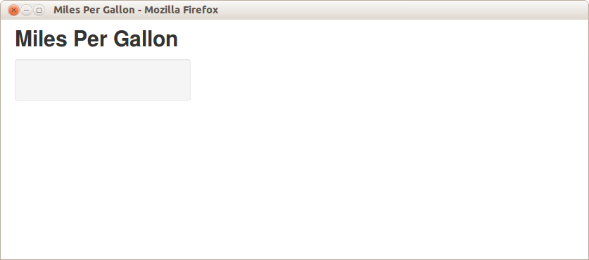
We now have a running Shiny application however it doesn’t do much yet. In the next section we’ll complete the application by specifying the user-interface and implementing the server script.
Inputs & Outputs
Adding Inputs to the Sidebar
The application we’ll be building uses the mtcars data from the R datasets package, and allows users to see a box-plot that explores the relationship between miles-per-gallon (MPG) and three other variables (Cylinders, Transmission, and Gears).
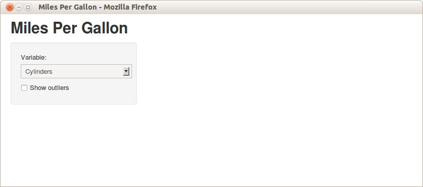
We want to provide a way to select which variable to plot MPG against as well as provide an option to include or exclude outliers from the plot. To do this we’ll add two elements to the sidebar, a selectInput to specify the variable and a checkboxInput to control display of outliers. Our user-interface definition looks like this after adding these elements:
ui.R
library(shiny)

# Define UI for miles per gallon application
shinyUI(pageWithSidebar(

  # Application title
  headerPanel("Miles Per Gallon"),

  # Sidebar with controls to select the variable to plot against mpg
  # and to specify whether outliers should be included
  sidebarPanel(
    selectInput("variable", "Variable:",
                list("Cylinders" = "cyl",
                     "Transmission" = "am",
                     "Gears" = "gear")),

    checkboxInput("outliers", "Show outliers", FALSE)
  ),

  mainPanel()
))
If you run the application again after making these changes you’ll see the two user-inputs we defined displayed within the sidebar:
Creating the Server Script
Next we need to define the server-side of the application which will accept inputs and compute outputs. Our server.R file is shown below, and illustrates some important concepts:
- Accessing input using slots on the
inputobject and generating output by assigning to slots on theoutputobject. - Initializing data at startup that can be accessed throughout the lifetime of the application.
- Using a reactive expression to compute a value shared by more than one output.
The basic task of a Shiny server script is to define the relationship between inputs and outputs. Our script does this by accessing inputs to perform computations and by assigning reactive expressions to output slots.
Here is the source code for the full server script (the inline comments explain the implementation technqiues in more detail):
server.R
library(shiny)
library(datasets)

# We tweak the "am" field to have nicer factor labels. Since this doesn't
# rely on any user inputs we can do this once at startup and then use the
# value throughout the lifetime of the application
mpgData <- mtcars
mpgData$am <- factor(mpgData$am, labels = c("Automatic", "Manual"))

# Define server logic required to plot various variables against mpg
shinyServer(function(input, output) {

  # Compute the forumla text in a reactive expression since it is
  # shared by the output$caption and output$mpgPlot expressions
  formulaText <- reactive({
    paste("mpg ~", input$variable)
  })

  # Return the formula text for printing as a caption
  output$caption <- renderText({
    formulaText()
  })

  # Generate a plot of the requested variable against mpg and only
  # include outliers if requested
  output$mpgPlot <- renderPlot({
    boxplot(as.formula(formulaText()),
            data = mpgData,
            outline = input$outliers)
  })
})
The use of renderText and renderPlot to generate output (rather than just assigning values directly) is what makes the application reactive. These reactive wrappers return special expressions that are only re-executed when their dependencies change. This behavior is what enables Shiny to automatically update output whenever input changes.
Displaying Outputs
The server script assigned two output values: output$caption and output$mpgPlot. To update our user interface to display the output we need to add some elements to the main UI panel.
In the updated user-interface definition below you can see that we’ve added the caption as an h3 element and filled in it’s value using the textOutput function, and also rendered the plot by calling the plotOutput function:
ui.R
library(shiny)

# Define UI for miles per gallon application
shinyUI(pageWithSidebar(

  # Application title
  headerPanel("Miles Per Gallon"),

  # Sidebar with controls to select the variable to plot against mpg
  # and to specify whether outliers should be included
  sidebarPanel(
    selectInput("variable", "Variable:",
                list("Cylinders" = "cyl",
                     "Transmission" = "am",
                     "Gears" = "gear")),

    checkboxInput("outliers", "Show outliers", FALSE)
  ),

  # Show the caption and plot of the requested variable against mpg
  mainPanel(
    h3(textOutput("caption")),

    plotOutput("mpgPlot")
  )
))
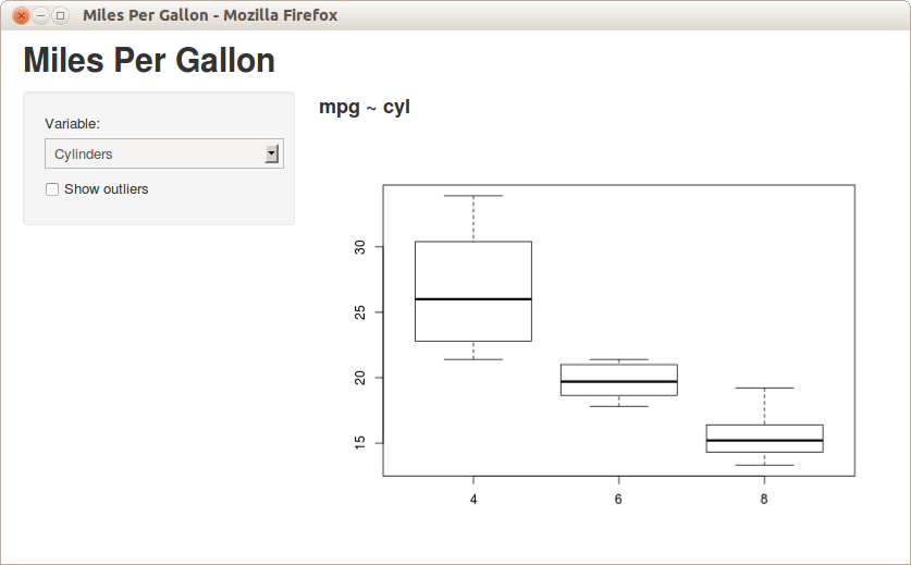
Running the application now shows it in its final form including inputs and dynamically updating outputs:
Now that we’ve got a simple application running we’ll probably want to make some changes. The next topic covers the basic cycle of editing, running, and debugging Shiny applications.
Run & Debug
Throughout the tutorial you’ve been calling runApp to run the example applications. This function starts the application and opens up your default web browser to view it. The call is blocking, meaning that it prevents traditional interaction with the console while the applciation is running.
To stop the application you simply interupt R – you can do this by pressing the Escape key in all R front ends as well as by clicking the stop button if your R environment provides one.
Running in a Separate Process
If you don’t want to block access to the console while running your Shiny application you can also run it in a separate process. You can do this by opening a terminal or console window and executing the following:
R -e "shiny::runApp('~/shinyapp')"
By default runApp starts the application on port 8100. If you are using this default then you can connect to the running application by navigating your browser to http://localhost:8100.
Note that below we discuss some techniques for debugging Shiny applications, including the ability to stop execution and inspect the current environment. In order to combine these techniques with running your applications in a separate terminal session you need to run R interactively (that is, first type “R” to start an R session then execute runApp from within the session).
Live Reloading
When you make changes to your underlying user-interface definition or server script you don’t need to stop and restart your application to see the changes. Simply save your changes and then reload the browser to see the updated application in action.
One qualification to this: when a browser reload occurs Shiny explicitly checks the timestamps of the ui.R and server.R files to see if they need to be re-sourced. If you have other scripts or data files that change Shiny isn’t aware of those, so a full stop and restart of the application is necessary to see those changes reflected.
Debugging Techniques
Printing
There are several techniques available for debugging Shiny applications. The first is to add calls to the cat function which print diagnostics where appropriate. For example, these two calls to cat print diagnostics to standard output and standard error respectively:
cat("foo\n")
cat("bar\n", file=stderr())
Using browser
The second technique is to add explicit calls to the browser function to interrupt execution and inspect the environment where browser was called from. Note that using browser requires that you start the application from an interactive session (as opposed to using R -e as described above).
For example, to unconditionally stop execution at a certain point in the code:
# Always stop execution here
browser()
You can also use this technique to stop only on certain conditions. For example, to stop the MPG application only when the user selects “Transmission” as the variable:
# Stop execution when the user selects "am"
browser(expr = identical(input$variable, "am"))
Establishing a custom error handler
You can also set the R "error" option to automatically enter the browser when an error occurs:
# Immediately enter the browser when an error occurs
options(error = browser)
Alternatively, you can specify the recover function as your error handler, which will print a list of the call stack and allow you to browse at any point in he stack:
# Call the recover function when an error occurs
options(error = recover)
If you want to set the error option automatically for every R session, you can do this in your .Rprofile file as described in this article on R Startup.
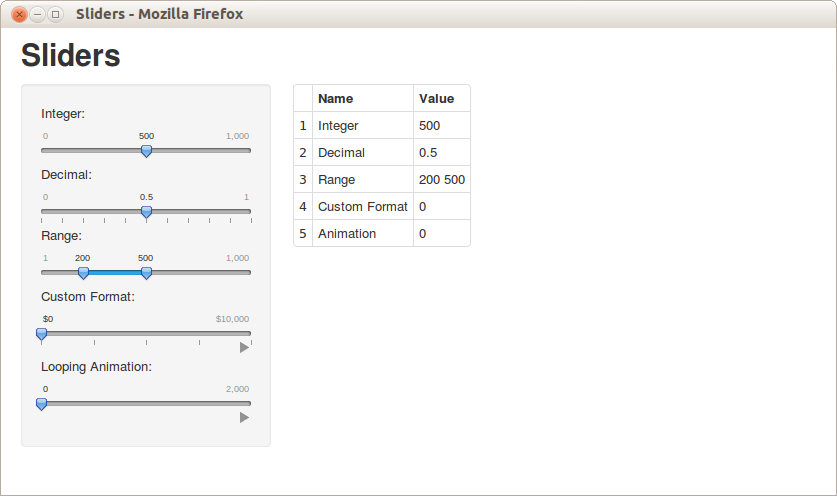
The Sliders application demonstrates the many capabilities of slider controls, including the ability to run an animation sequence. To run the example type:
> library(shiny)
> runExample("05_sliders")
Customizing Sliders
Shiny slider controls are extremely capable and customizable. Features supported include:
- The ability to input both single values and ranges
- Custom formats for value display (e.g for currency)
- The ability to animate the slider across a range of values
Slider controls are created by calling the sliderInput function. The ui.R file demonstrates using sliders with a variety of options:
ui.R
library(shiny)

# Define UI for slider demo application
shinyUI(pageWithSidebar(

  #  Application title
  headerPanel("Sliders"),

  # Sidebar with sliders that demonstrate various available options
  sidebarPanel(
    # Simple integer interval
    sliderInput("integer", "Integer:",
                min=0, max=1000, value=500),

    # Decimal interval with step value
    sliderInput("decimal", "Decimal:",
                min = 0, max = 1, value = 0.5, step= 0.1),

    # Specification of range within an interval
    sliderInput("range", "Range:",
                min = 1, max = 1000, value = c(200,500)),

    # Provide a custom currency format for value display, with basic animation
    sliderInput("format", "Custom Format:",
                min = 0, max = 10000, value = 0, step = 2500,
                format="$#,##0", locale="us", animate=TRUE),

    # Animation with custom interval (in ms) to control speed, plus looping
    sliderInput("animation", "Looping Animation:", 1, 2000, 1, step = 10,
                animate=animationOptions(interval=300, loop=T))
  ),

  # Show a table summarizing the values entered
  mainPanel(
    tableOutput("values")
  )
))
Server Script
The server side of the Slider application is very straightforward: it creates a data frame containing all of the input values and then renders it as an HTML table:
server.R
library(shiny)

# Define server logic for slider examples
shinyServer(function(input, output) {

  # Reactive expression to compose a data frame containing all of the values
  sliderValues <- reactive({

    # Compose data frame
    data.frame(
      Name = c("Integer",
               "Decimal",
               "Range",
               "Custom Format",
               "Animation"),
      Value = as.character(c(input$integer,
                             input$decimal,
                             paste(input$range, collapse=' '),
                             input$format,
                             input$animation)),
      stringsAsFactors=FALSE)
  })

  # Show the values using an HTML table
  output$values <- renderTable({
    sliderValues()
  })
})
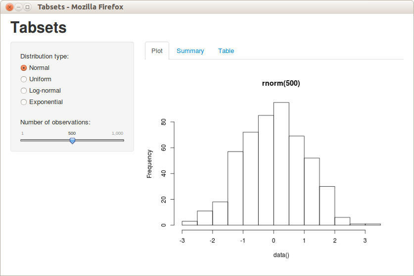
The Tabsets application demonstrates using tabs to organize output. To run the example type:
> library(shiny)
> runExample("06_tabsets")
Tab Panels
Tabsets are created by calling the tabsetPanel function with a list of tabs created by the tabPanel function. Each tab panel is provided a list of output elements which are rendered vertically within the tab.
In this example we updated our Hello Shiny application to add a summary and table view of the data, each rendered on their own tab. Here is the revised source code for the user-interface:
ui.R
library(shiny)

# Define UI for random distribution application
shinyUI(pageWithSidebar(

  # Application title
  headerPanel("Tabsets"),

  # Sidebar with controls to select the random distribution type
  # and number of observations to generate. Note the use of the br()
  # element to introduce extra vertical spacing
  sidebarPanel(
    radioButtons("dist", "Distribution type:",
                 list("Normal" = "norm",
                      "Uniform" = "unif",
                      "Log-normal" = "lnorm",
                      "Exponential" = "exp")),
    br(),

    sliderInput("n",
                "Number of observations:",
                 value = 500,
                 min = 1,
                 max = 1000)
  ),

  # Show a tabset that includes a plot, summary, and table view
  # of the generated distribution
  mainPanel(
    tabsetPanel(
      tabPanel("Plot", plotOutput("plot")),
      tabPanel("Summary", verbatimTextOutput("summary")),
      tabPanel("Table", tableOutput("table"))
    )
  )
))
Tabs and Reactive Data
Introducing tabs into our user-interface underlines the importance of creating reactive expressions for shared data. In this example each tab provides its own view of the dataset. If the dataset is expensive to compute then our user-interface might be quite slow to render. The server script below demonstrates how to calculate the data once in a reactive expression and have the result be shared by all of the output tabs:
server.R
library(shiny)

# Define server logic for random distribution application
shinyServer(function(input, output) {

  # Reactive expression to generate the requested distribution. This is
  # called whenever the inputs change. The renderers defined
  # below then all use the value computed from this expression
  data <- reactive({
    dist <- switch(input$dist,
                   norm = rnorm,
                   unif = runif,
                   lnorm = rlnorm,
                   exp = rexp,
                   rnorm)

    dist(input$n)
  })

  # Generate a plot of the data. Also uses the inputs to build the
  # plot label. Note that the dependencies on both the inputs and
  # the 'data' reactive expression are both tracked, and all expressions
  # are called in the sequence implied by the dependency graph
  output$plot <- renderPlot({
    dist <- input$dist
    n <- input$n

    hist(data(),
         main=paste('r', dist, '(', n, ')', sep=''))
  })

  # Generate a summary of the data
  output$summary <- renderPrint({
    summary(data())
  })

  # Generate an HTML table view of the data
  output$table <- renderTable({
    data.frame(x=data())
  })
})
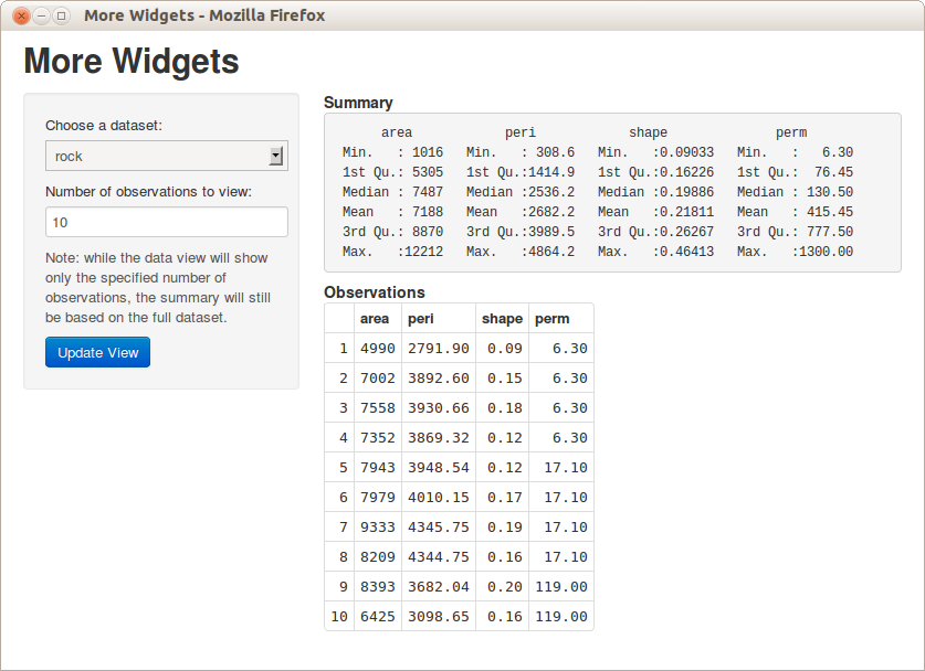
The More Widgets application demonstrates the help text and submit button widgets as well as the use of embedded HTML elements to customize formatting. To run the example type:
> library(shiny)
> runExample("07_widgets")
UI Enhancements
In this example we update the Shiny Text application with some additional controls and formatting, specifically:
- We added a
helpTextcontrol to provide additional clarifying text alongside our input controls. - We added a
submitButtoncontrol to indicate that we don’t want a live connection between inputs and outputs, but rather to wait until the user clicks that button to update the output. This is especially useful if computing output is computationally expensive. - We added
h4elements (heading level 4) into the output pane. Shiny offers a variety of functions for including HTML elements directly in pages including headings, paragraphics, links, and more.
Here is the updated source code for the user-interface:
ui.R
library(shiny)

# Define UI for dataset viewer application
shinyUI(pageWithSidebar(

  # Application title.
  headerPanel("More Widgets"),

  # Sidebar with controls to select a dataset and specify the number
  # of observations to view. The helpText function is also used to
  # include clarifying text. Most notably, the inclusion of a
  # submitButton defers the rendering of output until the user
  # explicitly clicks the button (rather than doing it immediately
  # when inputs change). This is useful if the computations required
  # to render output are inordinately time-consuming.
  sidebarPanel(
    selectInput("dataset", "Choose a dataset:",
                choices = c("rock", "pressure", "cars")),

    numericInput("obs", "Number of observations to view:", 10),

    helpText("Note: while the data view will show only the specified",
             "number of observations, the summary will still be based",
             "on the full dataset."),

    submitButton("Update View")
  ),

  # Show a summary of the dataset and an HTML table with the requested
  # number of observations. Note the use of the h4 function to provide
  # an additional header above each output section.
  mainPanel(
    h4("Summary"),
    verbatimTextOutput("summary"),

    h4("Observations"),
    tableOutput("view")
  )
))
Server Script
All of the changes from the original Shiny Text application were to the user-interface, the server script remains the same:
server.R
library(shiny)
library(datasets)

# Define server logic required to summarize and view the selected dataset
shinyServer(function(input, output) {

  # Return the requested dataset
  datasetInput <- reactive({
    switch(input$dataset,
           "rock" = rock,
           "pressure" = pressure,
           "cars" = cars)
  })

  # Generate a summary of the dataset
  output$summary <- renderPrint({
    dataset <- datasetInput()
    summary(dataset)
  })

  # Show the first "n" observations
  output$view <- renderTable({
    head(datasetInput(), n = input$obs)
  })
})
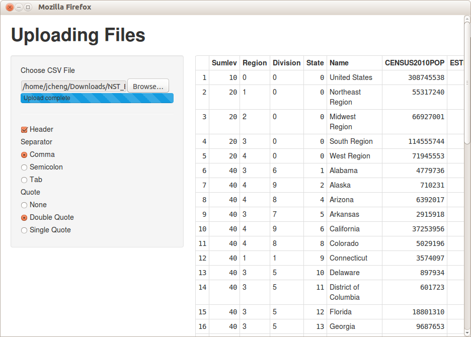
Sometimes you’ll want users to be able to upload their own data to your application. Shiny makes it easy to offer your users file uploads straight from the browser, which you can then access from your server logic.
Important notes:
- This feature does not work with Internet Explorer 9 and earlier (not even with Shiny Server).
- By default, Shiny limits file uploads to 5MB per file. You can modify this limit by using the
shiny.maxRequestSizeoption. For example, addingoptions(shiny.maxRequestSize=30*1024^2)to the top ofserver.Rwould increase the limit to 30MB.
To run this example, type:
> library(shiny)
> runExample("09_upload")
File upload controls are created by using the fileInput function in your ui.R file. You access the uploaded data similarly to other types of input: by referring to input$inputId. The fileInput function takes a multiple parameter that can be set to TRUE to allow the user to select multiple files, and an accept parameter can be used to give the user clues as to what kind of files the application expects.
ui.R
shinyUI(pageWithSidebar(
  headerPanel("CSV Viewer"),
  sidebarPanel(
    fileInput('file1', 'Choose CSV File',
              accept=c('text/csv', 'text/comma-separated-values,text/plain')),
    tags$hr(),
    checkboxInput('header', 'Header', TRUE),
    radioButtons('sep', 'Separator',
                 c(Comma=',',
                   Semicolon=';',
                   Tab='\t'),
                 'Comma'),
    radioButtons('quote', 'Quote',
                 c(None='',
                   'Double Quote'='"',
                   'Single Quote'="'"),
                 'Double Quote')
  ),
  mainPanel(
    tableOutput('contents')
  )
))
server.R
shinyServer(function(input, output) {
  output$contents <- renderTable({

    # input$file1 will be NULL initially. After the user selects and uploads a
    # file, it will be a data frame with 'name', 'size', 'type', and 'datapath'
    # columns. The 'datapath' column will contain the local filenames where the
    # data can be found.

    inFile <- input$file1

    if (is.null(inFile))
      return(NULL)

    read.csv(inFile$datapath, header=input$header, sep=input$sep, quote=input$quote)
  })
})
This example receives a file and attempts to read it as comma-separated values using read.csv, then displays the results in a table. As the comment in server.R indicates, inFile is either NULL or a dataframe that contains one row per uploaded file. In this case, fileInput did not have the multiple parameter so we can assume there is only one row.
The file contents can be accessed by reading the file named by the datapath column. See the ?fileInput help topic to learn more about the other columns that are available.
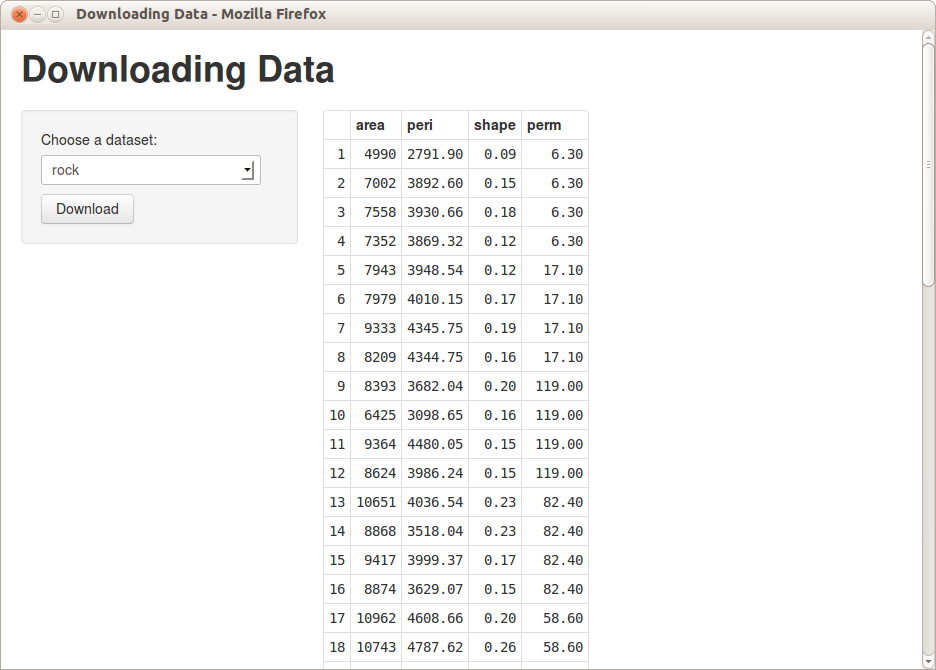
The examples so far have demonstrated outputs that appear directly in the page, such as plots, tables, and text boxes. Shiny also has the ability to offer file downloads that are calculated on the fly, which makes it easy to build data exporting features.
To run the example below, type:
> library(shiny)
> runExample("10_download")
You define a download using the downloadHandler function on the server side, and either downloadButton or downloadLink in the UI:
ui.R
shinyUI(pageWithSidebar(
  headerPanel('Download Example'),
  sidebarPanel(
    selectInput("dataset", "Choose a dataset:",
                choices = c("rock", "pressure", "cars")),
    downloadButton('downloadData', 'Download')
  ),
  mainPanel(
    tableOutput('table')
  )
))
server.R
shinyServer(function(input, output) {
  datasetInput <- reactive({
    switch(input$dataset,
           "rock" = rock,
           "pressure" = pressure,
           "cars" = cars)
  })

  output$table <- renderTable({
    datasetInput()
  })

  output$downloadData <- downloadHandler(
    filename = function() { paste(input$dataset, '.csv', sep='') },
    content = function(file) {
      write.csv(datasetInput(), file)
    }
  )
})
As you can see, downloadHandler takes a filename argument, which tells the web browser what filename to default to when saving. This argument can either be a simple string, or it can be a function that returns a string (as is the case here).
The content argument must be a function that takes a single argument, the file name of a non-existent temp file. The content function is responsible for writing the contents of the file download into that temp file.
Both the filename and content arguments can use reactive values and expressions (although in the case of filename, be sure your argument is an actual function; filename = paste(input$dataset, '.csv') is not going to work the way you want it to, since it is evaluated only once, when the download handler is being defined).
Generally, those are the only two arguments you’ll need. There is an optional contentType argument; if it is NA or NULL, Shiny will attempt to guess the appropriate value based on the filename. Provide your own content type string (e.g. "text/plain") if you want to override this behavior.
Dynamic UI
Shiny apps are often more than just a fixed set of controls that affect a fixed set of outputs. Inputs may need to be shown or hidden depending on the state of another input, or input controls may need to be created on-the-fly in response to user input.
Shiny currently has three different approaches you can use to make your interfaces more dynamic. From easiest to most difficult, they are:
- The
conditionalPanelfunction, which is used inui.Rand wraps a set of UI elements that need to be dynamically shown/hidden - The
renderUIfunction, which is used inserver.Rin conjunction with thehtmlOutputfunction inui.R, lets you generate calls to UI functions and make the results appear in a predetermined place in the UI - Use JavaScript to modify the webpage directly.
Let’s take a closer look at each approach.
Showing and Hiding Controls With conditionalPanel
conditionalPanel creates a panel that shows and hides its contents depending on the value of a JavaScript expression. Even if you don’t know any JavaScript, simple comparison or equality operations are extremely easy to do, as they look a lot like R (and many other programming languages).
Here’s an example for adding an optional smoother to a ggplot, and choosing its smoothing method:
# Partial example
checkboxInput("smooth", "Smooth"),
conditionalPanel(
  condition = "input.smooth == true",
  selectInput("smoothMethod", "Method",
              list("lm", "glm", "gam", "loess", "rlm"))
)
In this example, the select control for smoothMethod will appear only when the smooth checkbox is checked. Its condition is "input.smooth == true", which is a JavaScript expression that will be evaluated whenever any inputs/outputs change.
The condition can also use output values; they work in the same way (output.foo gives you the value of the output foo). If you have a situation where you wish you could use an R expression as your condition argument, you can create a reactive expression in server.R and assign it to a new output, then refer to that output in your condition expression. For example:
ui.R
# Partial example
selectInput("dataset", "Dataset", c("diamonds", "rock", "pressure", "cars")),
conditionalPanel(
  condition = "output.nrows",
  checkboxInput("headonly", "Only use first 1000 rows"))
server.R
# Partial example
datasetInput <- reactive({
   switch(input$dataset,
          "rock" = rock,
          "pressure" = pressure,
          "cars" = cars)
})

output$nrows <- reactive({
  nrow(datasetInput())
})
However, since this technique requires server-side calculation (which could take a long time, depending on what other reactive expressions are executing) we recommend that you avoid using output in your conditions unless absolutely necessary.
Creating Controls On the Fly With renderUI
Note: This feature should be considered experimental. Let us know whether you find it useful.
Sometimes it’s just not enough to show and hide a fixed set of controls. Imagine prompting the user for a latitude/longitude, then allowing the user to select from a checklist of cities within a certain radius. In this case, you can use the renderUI expression to dynamically create controls based on the user’s input.
ui.R
# Partial example
numericInput("lat", "Latitude"),
numericInput("long", "Longitude"),
uiOutput("cityControls")
server.R
# Partial example
output$cityControls <- renderUI({
  cities <- getNearestCities(input$lat, input$long)
  checkboxGroupInput("cities", "Choose Cities", cities)
})
renderUI works just like renderPlot, renderText, and the other output rendering functions you’ve seen before, but it expects the expression it wraps to return an HTML tag (or a list of HTML tags, using tagList). These tags can include inputs and outputs.
In ui.R, use a uiOutput to tell Shiny where these controls should be rendered.
Use JavaScript to Modify the Page
Note: This feature should be considered experimental. Let us know whether you find it useful.
You can use JavaScript/jQuery to modify the page directly. General instructions for doing so are outside the scope of this tutorial, except to mention an important additional requirement. Each time you add new inputs/outputs to the DOM, or remove existing inputs/outputs from the DOM, you need to tell Shiny. Our current recommendation is:
- Before making changes to the DOM that may include adding or removing Shiny inputs or outputs, call
Shiny.unbindAll(). - After such changes, call
Shiny.bindAll().
If you are adding or removing many inputs/outputs at once, it’s fine to call Shiny.unbindAll() once at the beginning and Shiny.bindAll() at the end – it’s not necessary to put these calls around each individual addition or removal of inputs/outputs.
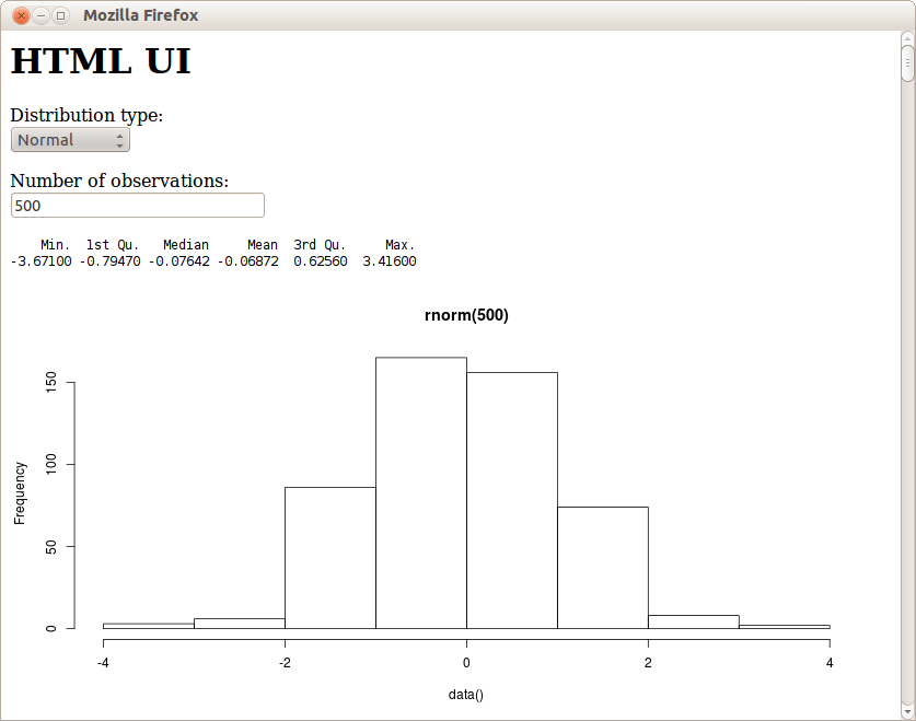
The HTML UI application demonstrates defining a Shiny user-interface using a standard HTML page rather than a ui.R script. To run the example type:
> library(shiny)
> runExample("08_html")
Defining an HTML UI
The previous examples in this tutorial used a ui.R file to build their user-interfaces. While this is a fast and convenient way to build user-interfaces, some appliations will inevitably require more flexiblity. For this type of application, you can define your user-interface directly in HTML. In this case there is no ui.R file and the directory structure looks like this:
<application-dir>
|-- www
    |-- index.html
|-- server.R
In this example we re-write the front-end of the Tabsets application using HTML directly. Here is the source code for the new user-interface definition:
www/index.html
<html>

<head>
  <script src="shared/jquery.js" type="text/javascript"></script>
  <script src="shared/shiny.js" type="text/javascript"></script>
  <link rel="stylesheet" type="text/css" href="shared/shiny.css"/>
</head>

<body>
  <h1>HTML UI</h1>

  <p>
    <label>Distribution type:</label><br />
    <select name="dist">
      <option value="norm">Normal</option>
      <option value="unif">Uniform</option>
      <option value="lnorm">Log-normal</option>
      <option value="exp">Exponential</option>
    </select>
  </p>

  <p>
    <label>Number of observations:</label><br />
    <input type="number" name="n" value="500" min="1" max="1000" />
  </p>

  <pre id="summary" class="shiny-text-output"></pre>

  <div id="plot" class="shiny-plot-output"
       style="width: 100%; height: 400px"></div>

  <div id="table" class="shiny-html-output"></div>
</body>

</html>
There are few things to point out regarding how Shiny binds HTML elements back to inputs and outputs:
- HTML form elmements (in this case a select list and a number input) are bound to input slots using their
nameattribute. - Output is rendered into HTML elements based on matching their
idattribute to an output slot and by specifying the requisite css class for the element (in this case either shiny-text-output, shiny-plot-output, or shiny-html-output).
With this technique you can create highly customized user-interfaces using whatever HTML, CSS, and JavaScript you like.
Server Script
All of the changes from the original Tabsets application were to the user-interface, the server script remains the same:
server.R
library(shiny)

# Define server logic for random distribution application
shinyServer(function(input, output) {

  # Reactive expression to generate the requested distribution. This is
  # called whenever the inputs change. The output renderers defined
  # below then all used the value computed from this expression
  data <- reactive({
    dist <- switch(input$dist,
                   norm = rnorm,
                   unif = runif,
                   lnorm = rlnorm,
                   exp = rexp,
                   rnorm)

    dist(input$n)
  })

  # Generate a plot of the data. Also uses the inputs to build the
  # plot label. Note that the dependencies on both the inputs and
  # the data reactive expression are both tracked, and all expressions
  # are called in the sequence implied by the dependency graph
  output$plot <- renderPlot({
    dist <- input$dist
    n <- input$n

    hist(data(),
         main=paste('r', dist, '(', n, ')', sep=''))
  })

  # Generate a summary of the data
  output$summary <- renderPrint({
    summary(data())
  })

  # Generate an HTML table view of the data
  output$table <- renderTable({
    data.frame(x=data())
  })
})
Scoping
Where you define objects will determine where the objects are visible. There are three different levels of visibility that you’ll want to be aware of when writing Shiny apps. Some objects are visible within the server.R code of each user session; other objects are visible in the server.R code across all sessions (multiple users could use a shared variable); and yet others are visible in the server.R and the ui.R code across all user sessions.
Per-session objects
In server.R, when you call shinyServer(), you pass it a function func which takes two arguments, input and output:
shinyServer(func = function(input, output) {
  # Server code here
  # ...
})
The function that you pass to shinyServer() is called once for each session. In other words, func is called each time a web browser is pointed to the Shiny application.
Everything within this function is instantiated separately for each session. This includes the input and output objects that are passed to it: each session has its own input and output objects, visible within this function.
Other objects inside the function, such as variables and functions, are also instantiated for each session. In this example, each session will have its own variable named startTime, which records the start time for the session:
shinyServer(function(input, output) {
  startTime <- Sys.time()

  # ...
})
Objects visible across all sessions
You might want some objects to be visible across all sessions. For example, if you have large data structures, or if you have utility functions that are not reactive (ones that don’t involve the input or output objects), then you can create these objects once and share them across all user sessions, by placing them in server.R, but outside of the call to shinyServer().
For example:
# A read-only data set that will load once, when Shiny starts, and will be
# available to each user session
bigDataSet <- read.csv('bigdata.csv')

# A non-reactive function that will be available to each user session
utilityFunction <- function(x) {
  # Function code here
  # ...
}

shinyServer(function(input, output) {
  # Server code here
  # ...
})
You could put bigDataSet and utilityFunction inside of the function passed to shinyServer(), but doing so will be less efficient, because they will be created each time a user connects.
If the objects change, then the changed objects will be visible in every user session. But note that you would need to use the <<- assignment operator to change bigDataSet, because the <- operator only assigns values in the local environment.
varA <- 1
varB <- 1
listA <- list(X=1, Y=2)
listB <- list(X=1, Y=2)

shinyServer(function(input, output) {
  # Create a local variable varA, which will be a copy of the shared variable
  # varA plus 1. This local copy of varA is not be visible in other sessions.
  varA <- varA + 1

  # Modify the shared variable varB. It will be visible in other sessions.
  varB <<- varB + 1

  # Makes a local copy of listA
  listA$X <- 5

  # Modify the shared copy of listB
  listB$X <<- 5

  # ...
})
Things work this way because server.R is sourced when you start your Shiny app. Everything in the script is run immediately, including the call to shinyServer()—but the function which is passed to shinyServer() is called only when a web browser connects and a new session is started.
Global objects
Objects defined in global.R are similar to those defined in server.R outside shinyServer(), with one important difference: they are also visible to the code in ui.R. This is because they are loaded into the global environment of the R session; all R code in a Shiny app is run in the global environment or a child of it.
In practice, there aren’t many times where it’s necessary to share variables between server.R and ui.R. The code in ui.R is run once, when the Shiny app is started and it generates an HTML file which is cached and sent to each web browser that connects. This may be useful for setting some shared configuration options.
Scope for included R files
If you want to split the server or ui code into multiple files, you can use source(local=TRUE) to load each file. You can think of this as putting the code in-line, so the code from the sourced files will receive the same scope as if you copied and pasted the text right there.
This example server.R file shows how sourced files will be scoped:
# Objects in this file are shared across all sessions
source('all_sessions.R', local=TRUE)

shinyServer(function(input, output) {
  # Objects in this file are defined in each session
  source('each_session.R', local=TRUE)

  output$text <- renderText({
    # Objects in this file are defined each time this function is called
    source('each_call.R', local=TRUE)

    # ...
  })
})
If you use the default value of local=FALSE, then the file will be sourced in the global environment.
Getting Non-Input Data From the Client
On the server side, Shiny applications use the input object to receive user input from the client web browser. The values in input are set by UI objects on the client web page. There are also non-input values (in the sense that the user doesn’t enter these values through UI components) that are stored in an object called session$clientData. These values include the URL, the pixel ratio (for high-resolution “Retina” displays), the hidden state of output objects, and the height and width of plot outputs.
Using session$clientData
To access session$clientData values, you need to pass a function to shinyServer() that takes session as an argument (session is a special object that is used for finer control over a user’s app session). Once it’s in there, you can access session$clientData just as you would input.
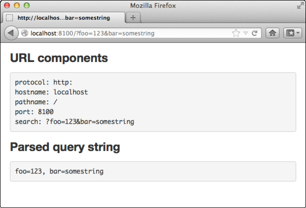
In the example below, the client browser will display out the components of the URL and also parse and print the query/search string (the part of the URL after a ”?”):
server.R
shinyServer(function(input, output, session) {

  # Return the components of the URL in a string:
  output$urlText <- renderText({
    paste(sep = "",
      "protocol: ", session$clientData$url_protocol, "\n",
      "hostname: ", session$clientData$url_hostname, "\n",
      "pathname: ", session$clientData$url_pathname, "\n",
      "port: ",     session$clientData$url_port,     "\n",
      "search: ",   session$clientData$url_search,   "\n"
    )
  })

  # Parse the GET query string
  output$queryText <- renderText({
    query <- parseQueryString(session$clientData$url_search)

    # Return a string with key-value pairs
    paste(names(query), query, sep = "=", collapse=", ")
  })
})
ui.R
shinyUI(bootstrapPage(
  h3("URL components"),
  verbatimTextOutput("urlText"),

  h3("Parsed query string"),
  verbatimTextOutput("queryText")
))
This app will display the following:
Viewing all available values in clientData
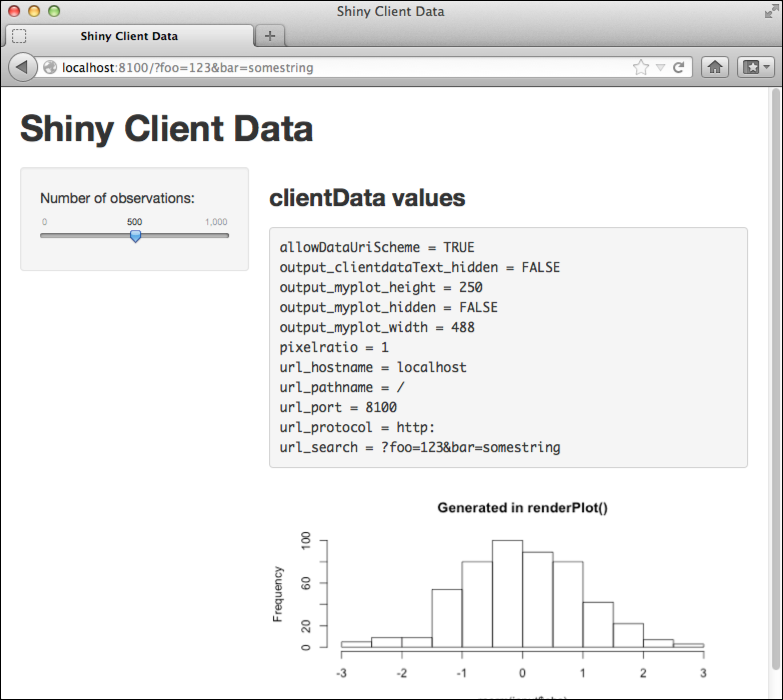
The values in session$clientData will depend to some extent on the outputs. For example, a plot output object will report its height, width, and hidden status. The app below has a plot output, and displays all the values in session$clientData:
shinyServer(function(input, output, session) {
  # Store in a convenience variable
  cdata <- session$clientData

  # Values from cdata returned as text
  output$clientdataText <- renderText({
    cnames <- names(cdata)

    allvalues <- lapply(cnames, function(name) {
      paste(name, cdata[[name]], sep=" = ")
    })
    paste(allvalues, collapse = "\n")
  })

  # A histogram
  output$myplot <- renderPlot({
    hist(rnorm(input$obs), main="Generated in renderPlot()")
  })
})
Notice that, just as with input, values in session$clientData can be accessed with session$clientData$myvar or session$clientData[['myvar']]. Or, equivalently, since we’ve saved it into a convenience variable cdata, we can use cdata$myvar or cdata[['myvar']].
ui.R
shinyUI(pageWithSidebar(
  headerPanel("Shiny Client Data"),
  sidebarPanel(
    sliderInput("obs", "Number of observations:",
                min = 0, max = 1000, value = 500)
  ),
  mainPanel(
    h3("clientData values"),
    verbatimTextOutput("clientdataText"),
    plotOutput("myplot")
  )
))
For the plot output output$myplot, there are three entries in clientData:
output_myplot_height: The height of the plot on the web page, in pixels.output_myplot_width: The width of the plot on the web page, in pixels.output_myplot_hidden: If the object is hidden (not visible), this is TRUE. This is used because Shiny will by default suspend the output object when it is hidden. When suspended, the observer will not execute even when its inputs change.
Here is the view from the client, with all the clientData values:
Sending Images
When you want to have R generate a plot and send it to the client browser, the renderPlot() function will in most cases do the job. But when you need finer control over the process, you might need to use the renderImage() function instead.
About renderPlot()
renderPlot() is useful for any time where R generates an image using its normal graphical device system. In other words, any plot-generating code that would normally go between png() and dev.off() can be used in renderPlot(). If the following code works from the console, then it should work in renderPlot():
png()
# Your plotting code here
dev.off()
# This would go in shinyServer()
output$myPlot <- renderPlot({
  # Your plotting code here
})
renderPlot() takes care of a number of details automatically: it will resize the image to fit the output window, and it will even increase the resolution of the output image when displaying on high-resolution (“Retina”) screens.
The limitation to renderPlot() is that it won’t send just any image file to the browser – the image must be generated by code that uses R’s graphical output device system. Other methods of creating images can’t be sent by renderPlot(). For example, the following won’t work:
- Image files generated by the
writePNG()function from the png package. - Image files generated by the
rgl.snapshot()function, which creates images from 3D plots made with the rgl package. - Images generated by an external program.
- Pre-rendered images.
The solution in these cases is the renderImage() function.
Using renderImage()
Image files can be sent using renderImage(). The expression that you pass to renderImage() must return a list containing an element named src, which is the path to the file. Here is a very basic example of a Shiny app with an output that generates a plot and sends it with renderImage():
server.R
shinyServer(function(input, output, session) {
  output$myImage <- renderImage({
    # A temp file to save the output.
    # This file will be removed later by renderImage
    outfile <- tempfile(fileext='.png')

    # Generate the PNG
    png(outfile, width=400, height=300)
    hist(rnorm(input$obs), main="Generated in renderImage()")
    dev.off()

    # Return a list containing the filename
    list(src = outfile,
         contentType = 'image/png',
         width = 400,
         height = 300,
         alt = "This is alternate text")
  }, deleteFile = TRUE)
})
ui.r
shinyUI(pageWithSidebar(
  headerPanel("renderImage example"),
  sidebarPanel(
    sliderInput("obs", "Number of observations:",
                min = 0, max = 1000,  value = 500)
  ),
  mainPanel(
    # Use imageOutput to place the image on the page
    imageOutput("myImage")
  )
))
Each time this output object is re-executed, it creates a new PNG file, saves a plot to it, then returns a list containing the filename along with some other values.
Because the deleteFile argument is TRUE, Shiny will delete the file (specified by the src element) after it sends the data. This is appropriate for a case like this, where the image is created on-the-fly, but it wouldn’t be appropriate when, for example, your app sends pre-rendered images.
In this particular case, the image file is created with the png() function. But it just as well could have been created with writePNG() from the png package, or by any other method. If you have the filename of the image, you can send it with renderImage().
Structure of the returned list
The list returned in the example above contains the following:
src: The output file path.contentType: The MIME type of the file. If this is missing, Shiny will try to autodetect the MIME type, from the file extension.widthandheight: The desired output size, in pixels.alt: Alternate text for the image.
Except for src and contentType, all values are passed through directly to the <img> DOM element on the web page. The effect is similar to having an image tag with the following:
<img src="..." width="400" height="300" alt="This is alternate text">
Note that the src="..." is shorthand for a longer URL. For browsers that support the data URI scheme, the src and contentType from the returned list are put together to create a special URL that embeds the data, so the result would be similar to something like this:
<img src="data:image/png;base64,iVBORw0KGgoAAAANSUhEUgAAAm0AAAGnCAYAAADlkGDxAAAACXBIWXMAAAsTAAALEwEAmpwYAAAgAElEQVR4nOydd3ic1ZX/P2+ZKmlU"
  width="400" height="300" alt="This is alternate text">
For browsers that don’t support the data URI scheme, Shiny sends a URL that points to the file.
Sending pre-rendered images with renderImage()
If your Shiny app has pre-rendered images saved in a subdirectory, you can send them using renderImage(). Suppose the images are in the subdirectory images/, and are named image1.jpeg, image2.jpeg, and so on. The following code would send the appropriate image, depending on the value of input$n:
server.R
shinyServer(function(input, output, session) {
  # Send a pre-rendered image, and don't delete the image after sending it
  output$preImage <- renderImage({
    # When input$n is 3, filename is ./images/image3.jpeg
    filename <- normalizePath(file.path('./images',
                              paste('image', input$n, '.jpeg', sep='')))

    # Return a list containing the filename and alt text
    list(src = filename,
         alt = paste("Image number", input$n))

  }, deleteFile = FALSE)
})
In this example, deleteFile is FALSE because the images aren’t ephemeral; we don’t want Shiny to delete an image after sending it.
Note that this might be less efficient than putting images in www/images and emitting HTML that points to the images, because in the latter case the image will be cached by the browser.
Using clientData values
In the first example above, the plot size was fixed at 400 by 300 pixels. For dynamic resizing, it’s possible to use values from session$clientData to detect the output size.
In the example below, the output object is output$myImage, and the width and height on the client browser are sent via session$clientData$output_myImage_width and session$clientData$output_myImage_height. This example also uses session$clientData$pixelratio to multiply the resolution of the image, so that it appears sharp on high-resolution (Retina) displays:
server.R
shinyServer(function(input, output, session) {

  # A dynamically-sized plot
  output$myImage <- renderImage({
    # Read myImage's width and height. These are reactive values, so this
    # expression will re-run whenever they change.
    width  <- session$clientData$output_myImage_width
    height <- session$clientData$output_myImage_height

    # For high-res displays, this will be greater than 1
    pixelratio <- session$clientData$pixelratio

    # A temp file to save the output.
    outfile <- tempfile(fileext='.png')

    # Generate the image file
    png(outfile, width=width*pixelratio, height=height*pixelratio,
        res=72*pixelratio)
    hist(rnorm(input$obs))
    dev.off()

    # Return a list containing the filename
    list(src = outfile,
         width = width,
         height = height,
         alt = "This is alternate text")
  }, deleteFile = TRUE)

  # This code reimplements many of the features of `renderPlot()`.
  # The effect of this code is very similar to:
  # renderPlot({
  #   hist(rnorm(input$obs))
  # })
})
The width and height values passed to png() specify the pixel dimensions of the saved image. These can differ from the width and height values in the returned list: those values are the pixel dimensions to used display the image. For high-res displays (where pixelratio is 2), a “virtual” pixel in the browser might correspond to 2 x 2 physical pixels, and a double-resolution image will make use of each of the physical pixels.
Reactivity Overview
It’s easy to build interactive applications with Shiny, but to get the most out of it, you’ll need to understand the reactive programming model used by Shiny.
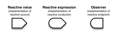
In Shiny, there are three kinds of objects in reactive programming: reactive sources, reactive conductors, and reactive endpoints, which are represented with these symbols:

Reactive sources and endpoints
The simplest structure of a reactive program involves just a source and an endpoint:

In a Shiny application, the source typically is user input through a browser interface. For example, when the selects an item, types input, or clicks on a button, these actions will set values that are reactive sources. A reactive endpoint is usually something that appears in the user’s browser window, such as a plot or a table of values.
In a simple Shiny application, reactive sources are accessible through the input object, and reactive endpoints are accessible through the output object. (Actually, there are other possible kinds of sources and endpoints, which we’ll talk about later, but for now we’ll just talk about input and output.)
This simple structure, with one source and one endpoint, is used by the 01_hello example. The server.R code for that example looks something like this:
shinyServer(function(input, output) {
  output$distPlot <- renderPlot({
    hist(rnorm(input$obs))
  })
})

You can see it in action at http://glimmer.rstudio.com/shiny/01_hello/.
The output$distPlot object is a reactive endpoint, and it uses the reactive source input$obs. Whenever input$obs changes, output$distPlot is notified that it needs to re-execute. In traditional program with an interactive user interface, this might involve setting up event handlers and writing code to read values and transfer data. Shiny does all these things for you behind the scenes, so that you can simply write code that looks like regular R code.
A reactive source can be connected to multiple endpoints, and vice versa. Here is a slightly more complex Shiny application:
shinyServer(function(input, output) {
  output$plotOut <- renderPlot({
    hist(faithful$eruptions, breaks = as.numeric(input$nBreaks))
    if (input$individualObs)
      rug(faithful$eruptions)
  })

  output$tableOut <- renderTable({
    if (input$individualObs)
      faithful
    else
      NULL
  })
})
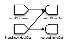
In a Shiny application, there’s no need to explictly describe each of these relationships and tell R what to do when each input component changes; Shiny automatically handles these details for you.
In an app with the structure above, whenever the value of the input$nBreaks changes, the expression that generates the plot will automatically re-execute. Whenever the value of the input$individualObs changes, the plot and table functions will automatically re-execute. (In a Shiny application, most endpoint functions have their results automatically wrapped up and sent to the web browser.)
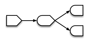
Reactive conductors
So far we’ve seen reactive sources and reactive endpoints, and most simple examples use just these two components, wiring up sources directly to endpoints. It’s also possible to put reactive components in between the sources and endpoints. These components are called reactive conductors.
A conductor can both be a dependent and have dependents. In other words, it can be both a parent and child in a graph of the reactive structure. Sources can only be parents (they can have dependents), and endpoints can only be children (they can be dependents) in the reactive graph.
Reactive conductors can be useful for encapsulating slow or computationally expensive operations. For example, imagine that you have this application that takes a value input$n and prints the nth value in the Fibonacci sequence, as well as the inverse of nth value in the sequence plus one (note the code in these examples is condensed to illustrate reactive concepts, and doesn’t necessarily represent coding best practices):
# Calculate nth number in Fibonacci sequence
fib <- function(n) ifelse(n<3, 1, fib(n-1)+fib(n-2))

shinyServer(function(input, output) {
  output$nthValue    <- renderText({ fib(as.numeric(input$n)) })
  output$nthValueInv <- renderText({ 1 / fib(as.numeric(input$n)) })
})
The graph structure of this app is:
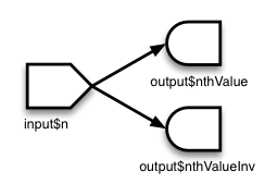
The fib() algorithm is very inefficient, so we don’t want to run it more times than is absolutely necessary. But in this app, we’re running it twice! On a reasonably fast modern machine, setting input$n to 30 takes about 15 seconds to calculate the answer, largely because fib() is run twice.
The amount of computation can be reduced by adding a reactive conductor in between the source and endpoints:
fib <- function(n) ifelse(n<3, 1, fib(n-1)+fib(n-2))

shinyServer(function(input, output) {
  currentFib         <- reactive({ fib(as.numeric(input$n)) })

  output$nthValue    <- renderText({ currentFib() })
  output$nthValueInv <- renderText({ 1 / currentFib() })
})
Here is the new graph structure:
Keep in mind that if your application tries to access reactive values or expressions from outside a reactive context — that is, outside of a reactive expression or observer — then it will result in an error. You can think of there being a reactive “world” which can see and change the non-reactive world, but the non-reactive world can’t do the same to the reactive world. Code like this will not work, because the call to fib() is not in the reactive world (it’s not in a reactive() or renderXX() call) but it tries to access something that is, the reactive value input$n:
shinyServer(function(input, output) {
  # Will give error
  currentFib      <- fib(as.numeric(input$n))
  output$nthValue <- renderText({ currentFib })
})
On the other hand, if currentFib is a function that accesses a reactive value, and that function is called within the reactive world, then it will work:
shinyServer(function(input, output) {
  # OK, as long as this is called from the reactive world:
  currentFib <- function() {
    fib(as.numeric(input$n))
  }

  output$nthValue <- renderText({ currentFib })
})
Summary
In this section, we’ve learned about:
- Reactive sources can signal objects downstream that they need to re-execute.
- Reactive conductors are placed somewhere in between sources and endpoints on the reactive graph. They are typically used for encapsulating slow operations.
- Reactive endpoints can be told to re-execute by the reactive environment, and can request upstream objects to execute.
- Invalidation arrows diagram the flow of invalidation events. It can also be said that the child node is a dependent of or takes a dependency on the parent node.
Implementations of sources, conductors, and endpoints: values, expressions, and observers
We’ve discussed reactive sources, conductors, and endpoints. These are general terms for parts that play a particular role in a reactive program. Presently, Shiny has one class of objects that act as reactive sources, one class of objects that act as reactive conductors, and one class of objects that act as reactive endpoints, but in principle there could be other classes that implement these roles.
- Reactive values are an implementation of Reactive sources; that is, they are an implementation of that role.
- Reactive expressions are an implementation of Reactive conductors. They can access reactive values or other reactive expressions, and they return a value.
- Observers are an implementation of Reactive endpoints. They can access reactive sources and reactive expressions, and they don’t return a value; they are used for their side effects.
All of the examples use these three implementations, as there are presently no other implementations of the source, conductor, and endpoint roles.
Reactive values
Reactive values contain values (not surprisingly), which can be read by other reactive objects. The input object is a ReactiveValues object, which looks something like a list, and it contains many individual reactive values. The values in input are set by input from the web browser.
Reactive expressions
We’ve seen reactive expressions in action, with the Fibonacci example above. They cache their return values, to make the app run more efficiently. Note that, abstractly speaking, reactive conductors do not necessarily cache return values, but in this implementation, reactive expressions, they do.
A reactive expressions can be useful for caching the results of any procedure that happens in response to user input, including:
- accessing a database
- reading data from a file
- downloading data over the network
- performing an expensive computation
Observers
Observers are similar to reactive expressions, but with a few important differences. Like reactive expressions, they can access reactive values and reactive expressions. However, they do not return any values, and therefore do not cache their return values. Instead of returning values, they have side effects – typically, this involves sending data to the web browser.
The output object looks something like a list, and it can contain many individual observers.
If you look at the code for renderText() and friends, you’ll see that they each return a function which returns a value. They’re typically used like this:
output$number <- renderText({ as.numeric(input$n) + 1 })
This might lead you to think that the observers do return values. However, this isn’t the whole story. The function returned by renderText() is actually not an observer/endpoint. When it is assigned to output$x, the function returned by renderText() gets automatically wrapped into another function, which is an observer. The wrapper function is used because it needs to do special things to send the data to the browser.
Differences between reactive expressions and observers
Reactive expressions and observers are similar in that they store expressions that can be executed, but they have some fundamental differences.
- Observers (and endpoints in general) respond to reactive flush events, but reactive expressions (and conductors in general) do not. We’ll learn more about flush events in the next section. If you want a reactive expression to execute, it must have an observer as a descendant on the reactive dependency graph.
- Reactive expressions return values, but observers don’t.
Execution scheduling
At the core of Shiny is its reactive engine: this is how Shiny knows when to re-execute each component of an application. We’ll trace into some examples to get a better understanding of how it works.
A simple example
At an abstract level, we can describe the 01_hello example as containing one source and one endpoint. When we talk about it more concretely, we can describe it as having one reactive value, input$obs, and one reactive observer, output$distPlot.
shinyServer(function(input, output) {
  output$distPlot <- renderPlot({
    hist(rnorm(input$obs))
  })
})
As shown in the diagram below, a reactive value has a value. A reactive observer, on the other hand, doesn’t have a value. Instead, it contains an R expression which, when executed, has some side effect (in most cases, this involves sending data to the web browser). But the observer doesn’t return a value. Reactive observers have another property: they have a flag that indicates whether they have been invalidated. We’ll see what that means shortly.
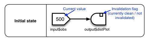
After you load this application in a web page, it be in the state shown above, with input$obs having the value 500 (this is set in the ui.r file, which isn’t shown here). The arrow represents the direction that invalidations will flow. If you change the value to 1000, it triggers a series of events that result in a new image being sent to your browser.
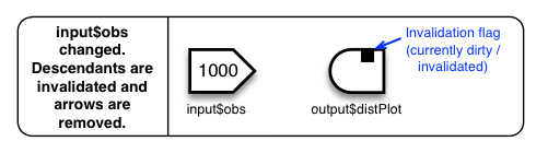
When the value of input$obs changes, two things happen:
- All of its descendants in the graph are invalidated. Sometimes for brevity we’ll say that an observer is dirty, meaning that it is invalidated, or clean, meaning that it is not invalidated.
- The arrows that have been followed are removed; they are no longer considered descendants, and changing the reactive value again won’t have any effect on them. Notice that the arrows are dynamic, not static.
In this case, the only descendant is output$distPlot:
Once all the descendants are invalidated, a flush occurs. When this happens, all invalidated observers re-execute.
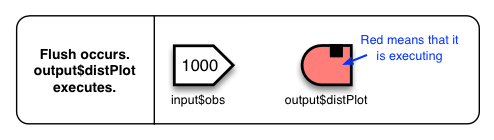
Remember that the code we assigned to output$distPlot makes use of input$obs:
output$distPlot <- renderPlot({
  hist(rnorm(input$obs))
})
As output$distPlot re-executes, it accesses the reactive value input$obs. When it does this, it becomes a dependent of that value, represented by the arrow . When input$obs changes, it invalidates all of its children; in this case, that’s justoutput$distPlot.
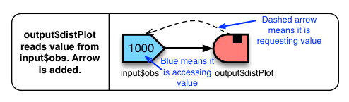
As it finishes executing, output$distPlot creates a PNG image file, which is sent to the browser, and finally it is marked as clean (not invalidated).
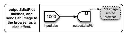
Now the cycle is complete, and the application is ready to accept input again.
When someone first starts a session with a Shiny application, all of the endpoints start out invalidated, triggering this series of events.
An app with reactive conductors
Here’s the code for our Fibonacci program:
fib <- function(n) ifelse(n<3, 1, fib(n-1)+fib(n-2))

shinyServer(function(input, output) {
  currentFib         <- reactive({ fib(as.numeric(input$n)) })

  output$nthValue    <- renderText({ currentFib() })
  output$nthValueInv <- renderText({ 1 / currentFib() })
})
Here’s the structure. It’s shown in its state after the initial run, with the values and invalidation flags (the starting value for input$n is set in ui.r, which isn’t displayed).
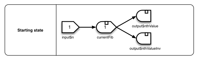
Suppose the user sets input$n to 30. This is a new value, so it immediately invalidates its children, currentFib, which in turn invalidates its children, output$nthValue and output$nthValueInv. As the invalidations are made, the invalidation arrows are removed:
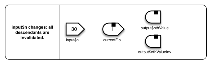
After the invalidations finish, the reactive environment is flushed, so the endpoints re-execute. If a flush occurs when multiple endpoints are invalidated, there isn’t a guaranteed order that the endpoints will execute, so nthValue may run before nthValueInv, or vice versa. The execution order of endpoints will not affect the results, as long as they don’t modify and read non-reactive variables (which aren’t part of the reactive graph).
Suppose in this case that nthValue() executes first. The next several steps are straightforward:
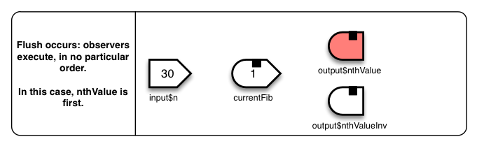
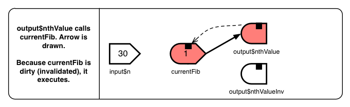
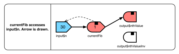
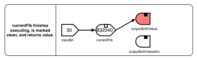
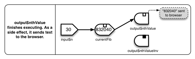
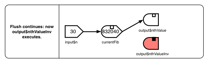
As output$nthValueInv() executes, it calls currentFib(). If currentFib() were an ordinary R expression, it would simply re-execute, taking another several seconds. But it’s not an ordinary expression; it’s a reactive expression, and it now happens to be marked clean. Because it is clean, Shiny knows that all of currentFib’s reactive parents have not changed values since the previous run currentFib(). This means that running the function again would simply return the same value as the previous run. (Shiny assumes that the non-reactive objects used by currentFib() also have not changed. If, for example, it called Sys.time(), then a second run of currentFib() could return a different value. If you wanted the changing values of Sys.time() to be able to invalidate currentFib(), it would have to be wrapped up in an object that acted as a reactive source. If you were to do this, that object would also be added as a node on the reactive graph.)
Acting on this assumption. that clean reactive expressions will return the same value as they did the previous run, Shiny caches the return value when reactive expressions are executed. On subsequent calls to the reactive expression, it simply returns the cached value, without re-executing the expression, as long as it remains clean.
In our example, when output$nthValueInv() calls currentFib(), Shiny just hands it the cached value, 832040. This happens almost instantaneously, instead of taking several more seconds to re-execute currentFib():
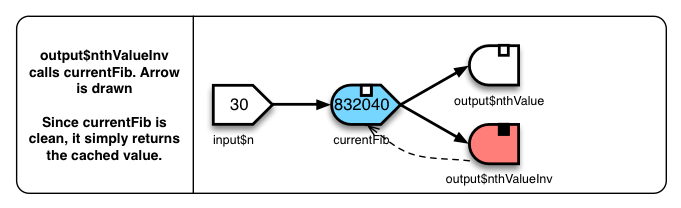
Finally, output$nthValueInv() takes that value, finds the inverse, and then as a side effect, sends the value to the browser.
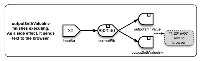
Summary
In this section we’ve learned about:
- Invalidation flags: reactive expressions and observers are invalidated (marked dirty) when their parents change or are invalidated, and they are marked as clean after they re-execute.
- Arrow creation and removal: After a parent object follows invalidates its children, the arrows will be removed. New arrows will be created when a reactive object accesses another reactive object.
- Flush events trigger the execution of endpoints. Flush events occur whenever the browser sends data to the server.
Isolation: avoiding dependency
Sometimes it’s useful for an observer/endpoint to access a reactive value or expression, but not to take a dependency on it. For example, if the observer performs a long calculation or downloads large data set, you might want it to execute only when a button is clicked.
For this, we’ll use actionButton. We’ll define a ui.R that is a slight modification of the one from 01_hello – the only difference is that it has an actionButton labeled “Go!”. You can see it in action at http://glimmer.rstudio.com/winston/actionbutton/.
The actionButton includes some JavaScript code that sends numbers to the server. When the web browser first connects, it sends a value of 0, and on each click, it sends an incremented value: 1, 2, 3, and so on.
shinyUI(pageWithSidebar(
  headerPanel("Click the button"),
  sidebarPanel(
    sliderInput("obs", "Number of observations:",
                min = 0, max = 1000, value = 500),
    actionButton("goButton", "Go!")
  ),
  mainPanel(
    plotOutput("distPlot")
  )
))
In our server.R, there are two changes to note. First, output$distPlot will take a dependency on input$goButton, simply by accessing it. When the button is clicked, the value of input$goButton increases, and so output$distPlot re-executes.
The second change is that the access to input$obs is wrapped with isolate(). This function takes an R expression, and it tells Shiny that the calling observer or reactive expression should not take a dependency on any reactive objects inside the expression.
shinyServer(function(input, output) {
  output$distPlot <- renderPlot({
    # Take a dependency on input$goButton
    input$goButton

    # Use isolate() to avoid dependency on input$obs
    dist <- isolate(rnorm(input$obs))
    hist(dist)
  })
})
The resulting graph looks like this:
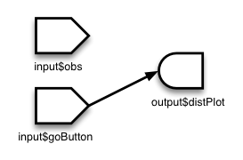
And here’s a walkthrough of the process when input$obs is set to 1000, and then the Go button is clicked:
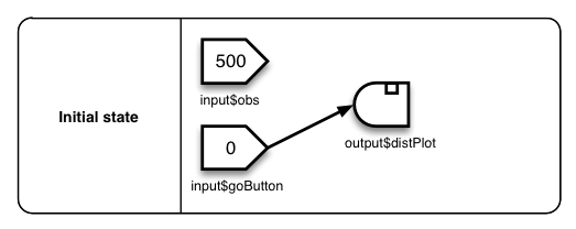
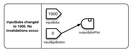
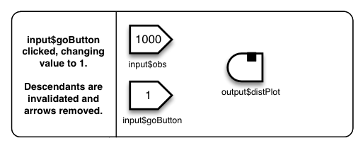
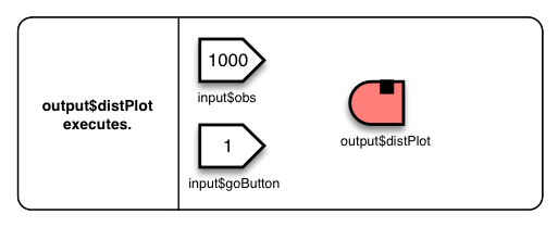

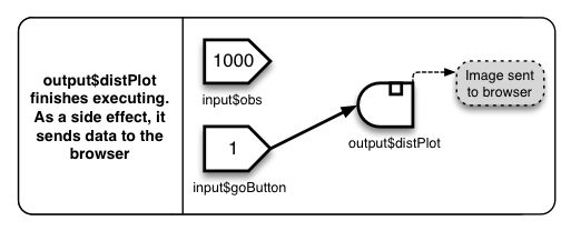
In the actionButton example, you might want to prevent it from returning a plot the first time, before the button has been clicked. Since the starting value of an actionButton is zero, this can be accomplished with the following:
  output$distPlot <- renderPlot({
    if (input$goButton == 0)
      return()

    # plot-making code here
  })
Reactive values are not the only things that can be isolated; reactive expressions can also be put inside an isolate(). Building off the Fibonacci example from above, this would calculate the nth value only when the button is clicked:
output$nthValue <- renderText({
  if (input$goButton == 0)
    return()

  isolate({ fib(as.numeric(input$n)) })
})
It’s also possible to put multiple lines of code in isolate(). For example here are some blocks of code that have equivalent effect:
# Separate calls to isolate -------------------------------
x <- isolate({ input$xSlider }) + 100
y <- isolate({ input$ySlider })  * 2
z <- x/y

# Single call to isolate ----------------------------------
isolate({
  x <- input$xSlider + 100
  y <- input$ySlider * 2
  z <- x/y
})

# Single call to isolate, use return value ----------------
z <- isolate({
  x <- input$xSlider + 100
  y <- input$ySlider * 2
  x/y
})
In all of these cases, the calling function won’t take a reactive dependency on either of the input variables.
Deploying Over the Web
Once you’ve written your Shiny app, you can make it available to anyone who has a web browser, using our Shiny Server software. You can either host the applications on your own server, or let us host your Shiny applications for you.
If you want a simple way to distribute your Shiny app so that users can run them on their own computers, see Deploying Shiny Apps to Run Locally.
Self-hosted Shiny Server
With our Shiny Server software, you can deploy Shiny applications over the web so that users need only a web browser and your application’s URL. You’ll need a Linux server and Shiny Server.
Shiny Server is free and open source, though in the future we will offer a commercially licensed edition with additional features for larger organizations. If you’d like to be notified of future beta releases of Shiny Server, please register now.
Pros
- Easiest for your users—only a web browser is required
- Take advantage of centralized computing resources
Cons
- Requires server setup and maintenance of a Linux server
RStudio-hosted Shiny Server
Want to deploy over the web but prefer not to run your own server? We’re currently beta testing a subscription-based hosting service for Shiny. To apply for a free beta test account, register now.
Pros
- Easiest for your users—only a web browser is required
- No need to run your own server
Cons
- Code and data must be copied to our servers
Sharing Apps to Run Locally
Once you’ve written your Shiny app, you can distribute it for others to run on their own computers—they can download and run Shiny apps with a single R command. This requires that they have R and Shiny installed on their computers.
If you want your Shiny app to be accessible over the web, so that users only need a web browser, see Deploying Shiny Apps over the Web.
Here are some ways to deliver Shiny apps to run locally:
Gist
One easy way is to put your code on gist.github.com, a code pasteboard service from GitHub. Both server.R and ui.R must be included in the same gist, and you must use their proper filenames. See https://gist.github.com/3239667 for an example.
Your recipient must have R and the Shiny package installed, and then running the app is as easy as entering the following command:
shiny::runGist('3239667')In place of '3239667' you will use your gist’s ID; or, you can use the entire URL of the gist (e.g. 'https://gist.github.com/3239667').
Pros
- Source code is easily visible by recipient (if desired)
- Easy to run (for R users)
- Easy to post and update
Cons
- Code is published to a third-party server
GitHub repository
If your project is stored in a git repository on GitHub, then others can download and run your app directly. An example repository is at https://github.com/rstudio/shiny_example. The following command will download and run the application:
shiny::runGitHub('shiny_example', 'rstudio')In this example, the GitHub account is 'rstudio' and the repository is 'shiny_example'; you will need to replace them with your account and repository name.
Pros
- Source code is easily visible by recipient (if desired)
- Easy to run (for R users)
- Very easy to update if you already use GitHub for your project
- Git-savvy users can clone and fork your repository
Cons
- Developer must know how to use git and GitHub
- Code is hosted by a third-party server
Zip File, delivered over the web
If you store a zip or tar file of your project on a web or FTP server, users can download and run it with a command like this:
runUrl('https://github.com/rstudio/shiny_example/archive/master.zip')The URL in this case is a zip file that happens to be stored on GitHub; replace it with the URL to your zip file.
Pros
- Only requires a web server for delivery
Cons
- To view the source, recipient must first download and unzip it
Zip File, copied to recipient’s computer
Another way is to simply zip up your project directory and send it to your recipient(s), where they can unzip the file and run it the same way you do (shiny::runApp).
Pros
- Share apps using e-mail, USB flash drive, or any other way you can transfer a file
Cons
- Updates to app must be sent manually
Package
If your Shiny app is useful to a broader audience, it might be worth the effort to turn it into an R package. Put your Shiny application directory under the package’s inst directory, then create and export a function that contains something like this:
shiny::runApp(system.file('appdir', package='packagename'))where appdir is the name of your app’s subdirectory in inst, and packagename is the name of your package.
Pros
- Publishable on CRAN
- Easy to run (for R users)
Cons
- More work to set up
- Source code is visible by recipient (if not desired)
Building Inputs
Shiny comes equipped with a variety of useful input components, but as you build more ambitious applications, you may find yourself needing input widgets that we don’t include. Fortunately, Shiny is designed to let you create your own custom input components. If you can implement it using HTML, CSS, and JavaScript, you can use it as a Shiny input!
(If you’re only familiar with R and not with HTML/CSS/JavaScript, then you will likely find it tough to create all but the simplest custom input components on your own. However, other people can – and hopefully will – bundle up their custom Shiny input components as R packages and make them available to the rest of the community.)
Design the Component
The first steps in creating a custom input component is no different than in any other form of web development. You write HTML markup that lays out the component, CSS rules to style it, and use JavaScript (mostly event handlers) to give it behavior, if necessary.
Shiny input components should try to adhere to the following principles, if possible:
- Designed to be used from HTML and R: Shiny user interfaces can either be written using R code (that generates HTML), or by writing the HTML directly. A well-designed Shiny input component will take both styles into account: offer an R function for creating the component, but also have thoughtfully designed and documented HTML markup.
- Configurable using HTML attributes: Avoid requiring the user to make JavaScript calls to configure the component. Instead, it’s better to use HTML attributes. In your component’s JavaScript logic, you can easily access these values using jQuery (or simply by reading the DOM attribute directly).
When used in a Shiny application, your component’s HTML markup will be repeated once for each instance of the component on the page, but the CSS and JavaScript will generally only need to appear once, most likely in the <head>. For R-based interface code, you can use the functions singleton and tags$head together to ensure these tags appear once and only once, in the head. (See the full example below.)
Write an Input Binding
Each custom input component also needs an input binding, an object you create that tells Shiny how to identify instances of your component and how to interact with them. (Note that each instance of the input component doesn’t need its own input binding object; rather, all instances of a particular type of input component share a single input binding object.)
An input binding object needs to have the following methods:
-
find(scope) -
Given an HTML document or element (
scope), find any descendant elements that are an instance of your component and return them as an array (or array-like object). The other input binding methods all take anelargument; that value will always be an element that was returned fromfind.A very common implementation is to use jQuery's
findmethod to identify elements with a specific class, for example:exampleInputBinding.find = function(scope) { return $(scope).find(".exampleComponentClass"); }; -
getId(el) -
Return the Shiny input ID for the element
el, ornullif the element doesn't have an ID and should therefore be ignored. The default implementation inShiny.InputBindingreads thedata-input-idattribute and falls back to the element'sidif not present. -
getValue(el) -
Return the Shiny value for the element
el. This can be any JSON-compatible value. -
setValue(el, value) - Set the element to the specified value. (This is not currently used, but in the future we anticipate adding features that will require the server to push input values to the client.)
-
subscribe(el, callback) -
Subscribe to DOM events on the element
elthat indicate the value has changed. When the DOM events fire, callcallback(a function) which will tell Shiny to retrieve the value.We recommend using jQuery's event namespacing feature when subscribing, as unsubscribing becomes very easy (see
unsubscribe, below). In this example,exampleComponentNameis used as a namespace:exampleInputBinding.subscribe = function(el, callback) { $(el).on("keyup.exampleComponentName", function(event) { callback(true); }); $(el).on("change.exampleComponentName", function(event) { callback(); }); };Later on, we can unsubscribe
".exampleComponentName"which will remove all of our handlers without touching anyone else's.The
callbackfunction optionally takes an argument: a boolean value that indicates whether the component's rate policy should apply (truemeans the rate policy should apply). SeegetRatePolicybelow for more details. -
unsubscribe(el) -
Unsubscribe DOM event listeners that were bound in
subscribe.Example:
exampleInputBinding.unsubscribe = function(el) { $(el).off(".exampleComponentName"); }; -
getRatePolicy() -
Return an object that describes the rate policy of this component (or
nullfor default).Rate policies are helpful for slowing down the rate at which input events get sent to the server. For example, as the user drags a slider from value A to value B, dozens of change events may occur. It would be wasteful to send all of those events to the server, where each event would potentially cause expensive computations to occur.
A rate policy slows down the rate of events using one of two algorithms (so far). Throttling means no more than one event will be sent per X milliseconds. Debouncing means all of the events will be ignored until no events have been received for X milliseconds, at which time the most recent event will be sent. This blog post goes into more detail about the difference between throttle and debounce.
A rate policy object has two members:
-
policy- Valid values are the strings"direct","debounce", and"throttle"."direct"means that all events are sent immediately. -
delay- Number indicating the number of milliseconds that should be used when debouncing or throttling. Has no effect if the policy isdirect.
Rate policies are only applied when the
callbackfunction insubscribeis called withtrueas the first parameter. It's important that input components be able to control which events are rate-limited and which are not, as different events may have different expectations to the user. For example, for a textbox, it would make sense to rate-limit events while the user is typing, but if the user hits Enter or focus leaves the textbox, then the input should always be sent immediately. -
Register Input Binding
Once you’ve created an input binding object, you need to tell Shiny to use it:
Shiny.inputBindings.register(exampleInputBinding, "yourname.exampleInputBinding");The second argument is a name the user can use to change the priority of the binding. On the off chance that the user has multiple bindings that all want to claim the same HTML element as their own, this call can be used to control the priority of the bindings:
Shiny.inputBindings.setPriority("yourname.exampleInputBinding", 10);Higher numbers indicate a higher priority; the default priority is 0. All of Shiny’s built-in input component bindings default to a priority of 0.
If two bindings have the same priority value, then the more recently registered binding has the higher priority.
Example
For this example, we’ll create a button that displays a number, whose value increases by one each time the button is clicked. Here’s what the end result will look like:
To start, let’s design the HTML markup for this component:
<button id="inputId" class="increment btn" type="button">0</button>The CSS class increment is what will differentiate our buttons from any other kind of buttons. (The btn class is just to make the button look decent in Twitter Bootstrap.)
Now we’ll write the JavaScript that drives the button’s basic behavior:
$(document).on("click", "button.increment", function(evt) {

  // evt.target is the button that was clicked
  var el = $(evt.target);

  // Set the button's text to its current value plus 1
  el.text(parseInt(el.text()) + 1);

  // Raise an event to signal that the value changed
  el.trigger("change");
});
This code uses jQuery’s delegated events feature to bind all increment buttons at once.
Now we’ll create the Shiny binding object for our component, and register it:
var incrementBinding = new Shiny.InputBinding();
$.extend(incrementBinding, {
  find: function(scope) {
    return $(scope).find(".increment");
  },
  getValue: function(el) {
    return parseInt($(el).text());
  },
  setValue: function(el, value) {
    $(el).text(value);
  },
  subscribe: function(el, callback) {
    $(el).on("change.incrementBinding", function(e) {
      callback();
    });
  },
  unsubscribe: function(el) {
    $(el).off(".incrementBinding");
  }
});

Shiny.inputBindings.register(incrementBinding);
Both the behavioral JavaScript code and the Shiny binding code should generally be run when the page loads. (It’s important that they run before Shiny initialization, which occurs after all the document ready event handlers are executed.)
The cleanest way to do this is to put both chunks of JavaScript into a file. In this case, we’ll use the path ./www/js/increment.js, which we can then access as http://localhost:8100/js/increment.js.
If you’re using an index.html style user interface, you’ll just need to add this line to your <head> (make sure it comes after the script tag that loads shiny.js):
<script src="js/increment.js"></script>On the other hand, if you’re using ui.R, then you can define this function before the call to shinyUI:
incrementButton <- function(inputId, value = 0) {
  tagList(
    singleton(tags$head(tags$script(src = "js/increment.js"))),
    tags$button(id = inputId,
                class = "increment btn",
                type = "button",
                as.character(value))
  )
}
Then in your shinyUI page definition you can call incrementButton wherever you want an increment button rendered. Notice the line that begins with singleton will ensure that the increment.js file will be included just one time, in the <head>, no matter how many buttons you insert into the page or where you place them.
Building Outputs
Right out of the box, Shiny makes it easy to include plots, simple tables, and text as outputs in your application; but we imagine that you’ll also want to display outputs that don’t fit into those categories. Perhaps you need an interactive choropleth map or a googleVis motion chart.
Similar to custom inputs, if you have some knowledge of HTML/CSS/JavaScript you can also build reusable, custom output components. And you can bundle up output components as R packages for other Shiny users to use.
Server-Side Output Functions
Start by deciding the kind of values your output component is going to receive from the user’s server side R code.
Whatever value the user’s R code returns is going to need to somehow be turned into a JSON-compatible value (Shiny uses RJSONIO to do the conversion). If the user’s code is naturally going to return something RJSONIO-compatible – like a character vector, a data frame, or even a list that contains atomic vectors – then you can just direct the user to use a function on the server. However, if the output needs to undergo some other kind of transformation, then you’ll need to write a wrapper function that your users will use instead (analogous to renderPlot or renderTable).
For example, if the user wants to output time series objects then you might create a renderTimeSeries function that knows how to translate ts objects to a simple list or data frame:
renderTimeSeries <- function(expr, env=parent.frame(), quoted=FALSE) {
    # Convert the expression + environment into a function
    func <- exprToFunction(expr, env, quoted)

    function() {
      val <- func()
      list(start = tsp(val)[1],
           end = tsp(val)[2],
           freq = tsp(val)[3],
           data = as.vector(val))
    }
}
which would then be used by the user like so:
output$timeSeries1 <- renderTimeSeries({
    ts(matrix(rnorm(300), 100, 3), start=c(1961, 1), frequency=12)
})
Design Output Component Markup
At this point, we’re ready to design the HTML markup and write the JavaScript code for our output component.
For many components, you’ll be able to have extremely simple HTML markup, something like this:
<div id="timeSeries1" class="timeseries-output"></div>
We’ll use the timeseries-output CSS class as an indicator that the element is one that we should bind to. When new output values for timeSeries1 come down from the server, we’ll fill up the div with our visualization using JavaScript.
Write an Output Binding
Each custom output component needs an output binding, an object you create that tells Shiny how to identify instances of your component and how to interact with them. (Note that each instance of the output component doesn’t need its own output binding object; rather, all instances of a particular type of output component share a single output binding object.)
An output binding object needs to have the following methods:
-
find(scope) -
Given an HTML document or element (
scope), find any descendant elements that are an instance of your component and return them as an array (or array-like object). The other output binding methods all take anelargument; that value will always be an element that was returned fromfind.A very common implementation is to use jQuery's
findmethod to identify elements with a specific class, for example:exampleOutputBinding.find = function(scope) { return $(scope).find(".exampleComponentClass"); }; -
getId(el) -
Return the Shiny output ID for the element
el, ornullif the element doesn't have an ID and should therefore be ignored. The default implementation inShiny.OutputBindingreads thedata-output-idattribute and falls back to the element'sidif not present. -
renderValue(el, data) - Called when a new value that matches this element's ID is received from the server. The function should render the data on the element. The type/shape of the `data` argument depends on the server logic that generated it; whatever value is returned from the R code is converted to JSON using the RJSONIO package.
-
renderError(el, err) -
Called when the server attempts to update the output value for this element, and an error occurs. The function should render the error on the element.
erris an object with amessageString property. -
clearError(el) -
If the element
elis currently displaying an error, clear it.
Register Output Binding
Once you’ve created an output binding object, you need to tell Shiny to use it:
Shiny.outputBindings.register(exampleOutputBinding, "yourname.exampleOutputBinding");
The second argument is a string that uniquely identifies your output binding. At the moment it is unused but future features may depend on it.